Text Mining and Analytics

by ChengXiang Zhai

CONTENT

1. Overview Text Mining and Analysis
2. Natural Language Processing & Text Representation
3. Word Association Mining and Analysis
     └ Paradigmatic
     └ Syntagmatic


7. Topic Mining and Analysis
8. Probabilistic Topic Models
9. Probabilistic Latent Semantic Analysis (PLSA)
10. Latent Dirichlet Allocation (LDA)
11. Text Clustering
12. Text Categorization
13. Opinion Mining and Sentiment Analysis
14. Latent Aspect Rating Analysis
15. Text-Based Prediction
16. Contextual Text Mining


3. Word Association Mining and Analysis

3.1 Paradigmatic Relation Discovery
ㆍParadigmatic Relation
A & B have paradigmatic relation if they can be substituted for each other (i.e., A & B are in the same class)

3.2. Syntagmatic Relation Discovery
In semiotics, syntagmatic analysis is analysis of syntax or surface structure (syntagmatic structure) as opposed to paradigms (paradigmatic analysis). This is often achieved using commutation tests. Syntagmatic means one element selects the other element either to precede it or to follow it. For example, the definitive article "the" selects a noun and not a verb.

ㆍSyntagmatic Relation = Correlated Occurrences
A & B have syntagmatic relation if they can be combined with each other.(i.e., A & B are related semantically)
When we see one word occurs in context, we tend to see the occurrence of the other word in the same text segment. For example, whenever "eats" occurs, what other words also tend to occur? What words tend to occur the left of "eats"? and What words are to the right?. In other words, what other words are associated with "eats"? If they are associated with "eats", they tend to occur in the context of "eats".

ㆍWord Prediction Problem
Is word W present(or absent) in this text segment(any unit, e.g., sentence, paragraph, document?. Among "meat", "the", "unicorn", what word is the easiest to predict than others? The "meat" is hard to predict because it might be present or absent in any text segment. The "the or "unicorn" is easy to predict because "the" must be present and "unicorn" should be rarely in text segment.
The harder to predict, the higher the entropy is and
The easier to predict, the lower the entropy is.

The problem can be formally defined as predicting the value of a binary random variable, $X_w$ which is associated with precisely one word. The intuition with this concept is that the more random $X_w$ is, the more difficult the prediction would be.  
Now, the question is how does one quantitatively measure the randomness of a random variable like $X_w$? ( Assuming that there is no statistic or sample space which can measure the probability of presenting word w )

3.2.1. Entropy
In order to quantitatively measure the randomness of X, we'll use Entropy from Information Theory. For our purpose, we'll just treat entropy function as a function defined on a binary random variable like this:

This entropy function will give a different value for different distributions of this random variable and it clearly depends on the probability that the random variable taking value of 1 or 0. The entropy function look like this:

For what $X_w$, does $H($X_w$)$ reach maximum/minimum?
For example, In Coin tossing, we can think two cases, fair coin and completely biased coin. First, Fair coin has P(X=1)=P(X=0)=1/2 and so $H(X)$ = -1/2$log_2$1/2 -1/2$log_2$1/2=1. Second, Completely biased coin has P(X=1)=1 and so $H(X)$=-0*$log_2$0-1*$log_2$1=0. Thus, since Fair coin is most difficult to predict, it has the highest entropy value.

So, how can we use entropy for word prediction? The problem is to predict word w is present or absent in the text segment. We can assume high entropy words are harder to predict. We now have a quantitative way to tell us which word is harder to predict. Now if you look at the three words meat, the, and unicorn, then we clearly would expect meat to have a higher entropy than others.

3.2.2 Conditional Entropy
We assume that we know something about the text segment. That is, given that we know that "eats" occurred in the text segment, how would that help us predict the presence or absence of "meat"? In particular, we want to know whether the presence of "eats" has help us predict the presence of "meat". In other words, the presence of "eats" could reduce uncertainty about "meat"? or reduce the entropy of the random variable?
These questions can be addressed by using Conditional Entropy implemented with conditional probabilities rather than probabilities.

In general, for any discrete random variables X and Y, the conditional entropy is no larger than the entropy itself. Therefore, $H(X)$ is upper bound for the $H(X|Y)$, which means as we know more information such as Y, we tend to reduce uncertainty(or Entropy) because the information, Y should always help us make the prediction.

Example of Conditional Entropy to capture Syntagmatic Relation
- $H($X_(meat)$|$X_(meat)$)$ = 0, which means we're already know the answer of the prediction
- $H($X_(meat)$|$X_(the)$)$ ≒ $H($X_(meat)$)$, which means knowing the occurrence of "the" doesn't really help us reduce entropy that much so it stays fairly close to the original entropy of "meat".
- $H($X_(meat)$|$X_(eats)$)$, which means since there is a strong association between "meat" and "eats" (i.e, knowing presence or absence of "eats" help us to predict whether "meat" occurs), it becomes smaller entropy. Therefore, The conditional entropy gives us directly a way to measure the association of two words.
For which word w, does $H($X_(meat)$|$X_w$)$ reach its minimum or maximum? It depends on the degree of relation between them.

Conditional Entropy for Mining Syntagmatic Relations ( Algorithm View )
ㆍFor each word $W_1$
   - For every other word $W_2$, compute conditional entropy $H($X_(w1)$|$X_(w2)$)$
   - Sort all the candidate words in ascending order of $H($X_(w1)$|$X_(w2)$)$
   - Take the top-ranked candidate words as words that have potential syntagmatic relations with w1
   - Need to use a threshold for each w1

This would allow us to mine the most strongly correlated words with a particular word, w1. However, this algorithm does not help us mine the strongest that K sysntagmatical relations from an entire collection because we can't ensure that these conditional entropies are comparable across different words. For example, while $H($X_(w1)$|$X_(w2)$)$ and $H($X_(w1)$|$X_(w3)$)$ are comparable (i.e., they all measure how hard it is to predict w1), $H($X_(w1)$|$X_(w2)$)$ and $H($X_(w3)$|$X_(w2)$)$ aren't because they have different upper bounds which are the entropy of w1 and w3. (We only need word association mining to discover syntagmatic relation so we don't need to care about their position (left or right). But, Conditional Entropy consider that left-side of word which determine upper bound, is major.)

The problem of conditional entropy which cannot be comparable to compute different pairs of words, makes it harder to discover strong syntagmatic relations globally from corpus. How do we address this problem? we can use Mutual Information to solve this problem of conditional entropy.

3.2.3. Mutual Information
It allows  us to normalize the conditional entropy to make it more comparable across different pairs by measuring Entropy Reduction. The philosophy is how much reduction in the entropy of X can we obtain by knowing Y. Mutual Information is defined as:

Even though the two conditional entropies are not equal, interestingly the reduction of entropy by knowing one of them is actually equal. This reduction quantity is called a Mutual Information denoted by I(X; Y).

It has several interesting properties.
- Non-negative ( I(X; Y) ≥ 0 ) because Conditional entropy will never exceed the original entropy. Knowing some information can always help us potentially, but will not hurt us in predicting X.
- Symmetric ( I(X; Y)=I(Y; X) )
- I(X; Y)=0 iff X & Y are independent, which means knowing one of them does not tell us anything about the other.

When we fix X to rank different Ys, I(X; Y) and H(X| Y) give the same order, but I(X; Y) allows us to compare different (X, Y) pairs, which is more general and useful to use Mutual Information.

Mutual Information for Mining Syntagmatic Relations
Whenever "eats" occurs, what other words also tend to occur? (Which words have high mutual information with "eats"?) By computing Mutual information between two words, we can see how strongly associated two words are. The more related two words are, the higher Mutual Information is.

Knowing "the" does not really help us to predict the presence of "eats" and vice versa.
$I(X_(eats);X_(eats))$ is maximum because knowing one allows us to predict the other completely. and then conditional entropy is zero therefore, mutual information(reduction) is maximum.








Topic Mining and Analysis: 
Motivation and Task Definition

Topic Mining (or Content Mining) : trying to discover knowledge about the main topics in the text.

Motivation

• Topic is similar with the main idea discussed in text data, or theme/subject of a discussion or conversation.
• Topic can indicate the different granularities (새로운 단위) (e.g., topic of a sentence, an article, topic of paragraph, topic of all the research articles in the research library) 
• Topics as knowledge about the world: topics generally provide a description about the world, they tell us something about the world. (Text+Non-text data를 이용해 역으로 추론이 가능하다.)

IDEA : Topic =  Word Distribution

• Word Distribution represents a topic if we assemble words from the distribution we tended to see words that are ready to dispose.
• It uses multiple words to describe a topic so it allows us to describe a fairly complicated topics.
• It assigns weights to terms, now we can model several differences of semantics and you can bring in related words together to model a topic.
• Since we have probabilities for the same word in different topics, we can disintegrate the sense of word. Topic들 간에서 sharing하는 word들도 물론 존재한다. 대신 각자의 sample space에서의 확률은 다르다.
• In a very special case, if the probability of mass is concentrated entirely on just one word and it means the symbol foundation of a topic was just one word. ( 'Topic=Word' is a special case of 'Topic=Word Distribution' )  하지만, 거의 대부분 Word Distribution으로 표현한다. 이처럼 많은 단어들을 사용하여 topic의 미묘한 차이까지 modeling한다.
• Vocabulary set을 사용하기 때문에 Topic과 완전히 관련없는 단어들이더라도 non-zero probability를 유지한다.

Generative Model for Text Mining

It's a principle way of using statistical modeling to solve text mining. First, we design a model with some parameter values to fit the data as well as we can (1.Modeling of Data Generation). Second, after we have fit the data, we will recover some parameter values. (2.Parameter Estimation/Inferences). those would be the outcome of the algorithm and we'll treat these as the discovered knowledge from text data.

 1. Modeling of Data Generation

• The idea of this approach is actually to first design a model for our data. So we design a probabilistic model to model how the data are generated. ( this is based on our assumption. the actual data aren't necessarily generating in this way. ) 
• 여기서는 우리가 parameter를 사용해서 Model을 만들어 data들이 나의 Model 기반 위에서 있다고 가정한다. Gaussian Distribution 모델을 사용하면, 간단하게 식을 대입하면 된다.
• We have a set of 's which is all word distribution
• We have a set of 's for each document
• Since we have n documents, we need to have n sets of Pis and each Pi value sum to 1.
• This is to say that we first would pretend that we already have these word distributions and the coverage numbers.
• Now, we can see how we can generate data by using such distributions.
• But, how do we model the data in this way ?

ASSUMPTION : the data are actual samples drawn from such a model that depends on these parameters.

* Lambda : this template consists of all the parameters that we're interested in and that will control the behavior of the probabilistic model.


2. Parameter Estimation/ Inferences

• Once we set up the model, we can fit the model to our data.
• We can estimate the parameters or infer the parameters based on the data.
• We'd like to adjust these parameter values until we give our data set the maximum probability.

Simple version

• What parameter values will give our data set the highest probability ? It's * which is our estimate of the parameters and which is precisely what we hoped to discover from text data. and we'd treat it as the outcome.

Overview of Statistical Language Models

Statistical Language Model

• A probability distribution over word sequences ( context-dependent )
• ex. P("Today is Wednesday")=0.001, P("Today Wednesday is")=0.0000000001
• It can also be regarded as a probabilistic mechanism for 'generating' text - thus also called a 'generative' model.
• Given a model, we can sample the sequence of the words.

하지만, 모든 경우의 수의 word들의 sequence를 나타내는 것은 매우 값비싼 computation(거의 불가능)이므로, model을 좀 더 'Simple'하게 만들 필요가 있다.

The Simplest Language Model: Unigram LM

• Generate text by generating each word independently
• Thus, P(w1, w2, ... wn) = P(w1)P(w2)...P(wn); sequence의 확률을 단순히 각개의 word들의 확률 곱으로 나타낸다.
• Text = sample drawn according to this word distribution

Independent Assumption의 힘 : each word distribution으로 모든 word sequence의 distribution을 나타낼 수 있다. 하지만, sequence의 order(순서)는 ignore해버린다. 그래도 좋은 approximation이 될 수 있다.

When we have a model, we generally have two problems.
1. Given a model how likely we observe certain kind of data points, that is, we are interested in Sampling Process.

• No word has 0 probability, we can essentially generate all kind of text documents.
• Text mining Model은 특히, Text mining paper는 높은 확률로 generate할 수 있다. 반면, Food nutrition paper는 낮은 확률로 generate한다. 특정 Topic 중심으로 Modeling한 Unigram LM이더라도, 모든 문서를 generation할 수 있긴 있다. 단지, 매우 다양한 확률 분포를 가질 뿐이다.

2. Estimation Process, figure out parameter given observed data.

• Real World에서는 항상 Sample Data만 얻을 수 있다. 즉, 인터넷상에서 Text Mining 주제 섹션에 있는 Paper 한장을 획득하였다. 
• Estimation: 우리는 Sample Data만으로 전체(Population)을 보는 눈이 필요하다. 
• 간단히, Count를 통해 Sample 표본에서의 Word들의 확률을 구하여 Maximum Likelihood Estimate 기법을 사용해 LM을 Estimation할 수 있다. 하지만, 이러한 Estimation이 Best한가 ? 

Real World에서 우리가 가질 수 밖에 없는 Sample을 통해 최대한 비슷하게 전체(Population)를 보는 눈을 어떻게 가질 수 있을까? (= 어떻게 Estimation을 할 것인가.)


Maximum Likelihood Estimation

• "Best" means "data likelihood reaches maximum"
• PROBLEM : Sample size가 작으면, Bias되기 쉽다. ( 단편적인면만 보기 때문에..) 그리고 Sample에 없는 단어들을 non-zero probability로 처리하는데 아무래도 optimal하지 않고, 정확성이 떨어진다. (새로운 정보(prior)가 필요..)

Bayesian Estimation (or Maximum a Posterior Estimate)

• "Best" means being consistent with our "prior" knowledge and explaining data well.
• data뿐만 아니라 prior까지 고려한다. we'll impose some preference on certain theta's of others.
• P(Theta|X) represents a compromise of the two parameters.
• MAP estimate is more general than Maximum likelihood because if we define our prior as a non-informative prior, meaning that it's uniform over all the theta values, no preference, then we basically would go back to the Maximum likelihood estimation. but if we have informative prior or bias towards the different values, then MAP estimation can allow us to incorporate that.
• PROBLEM : How to define prior?

Bayes Rule

1. Posterior Belief ( P(X | Y) ) : this is our belief about X values after we have observed the Y. Now, do we believe some values have higher probability than others?
2. Prior Belief ( P(X) ) : We assume that we have some prior belief about the parameter. before we observe any other data, this is our belief about X. by using prior belief, what we strongly believe can have higher probability than others. (데이터를 수집하기 전, 이미 믿고 있는 확률)

• After we have observed Y, we'll update our belief and the updating formula is based on the combination of our prior and the likelihood of observing this Y if X is indeed true.

Illustration of Bayesian Estimation

1. Posterior : to compromise between Likelihood and Prior; P(theta|X)와 P(X|theta)P(theta)는 서로 크기가 다를 진 몰라도 서로 비례관계에 있으므로 maximum이 되게하는 theta값은 서로 같다.
2. Likelihood : this theta value can best expand our data.(only data)
3. Prior : you'll see this can be useful for topic mining where we want to inject the sum prior knowledge about the topics. ( 이 정보도 이제 같이 고려하겠다. )
4. Prior Mode : the most likely parameter value according to our prior before we observe any data.
5. Posterior Mode : it's the most likely value of theta given by the posterior distribution and it represents a good compromise between the prior mode and the maximum likelihood estimate.

Topic Mining and Analysis: 
Mixture of Unigram Language Models

Motivation

일반 Document의 word count로 Distribution을 나타내면, common word(the, a,..)들의 확률이 제일 높게 나온다. these common words should not be explained by this distribution. One natural way to solve this problem is to think about using another distribution(Background distribution) to account for these common words. In this way, the two distributions can be mixed together to generate the text data.   

The Idea of a Mixture Model

• d (Topic) : only to generate the content words 
• B (Background) : to generate the common words
• P(d)+P(B) =1; 여기서는 새로운 정보가 없으므로 가장 이상적인 확률인 0.5이지만, 보통 한쪽으로 Bias된다. 
• Although we have a mixture model that has some uncertainty associated with the use of two word distributions, we can still think of this as a model for generating text data because each word will still be a sample from one of two distributions.
• If we view this whole box as one model, it's just like generative model(일반적으로 1개의 distribution을 가짐) in that giving us the probability of a word.
• We can treat this as a generative model and it's often useful to think of just as a likelihood.

As a Generative Model

1. Setup a Mixture Model
2. Generative model or Likelihood function
3. Estimate the parameters

• the mixture model is more general than the previous model where we have just one distribution. the mixture model can cover one distribution as a special case.
• We can use observed text data to estimate the model parameters. this estimation would allow us to discover the interesting knowledge about the text. 
• Interesting Knowledge (parameters) : two word distributions that result in topics, the coverage of each topic.

Mixture of Two Unigram Language Models

• Likelihood function : By using a product over all the unique words in our vocabulary instead of all the positions in the document. the form where we look at the different and unique words, is convenient form for computing maximum likelihood estimate.
• Lambda notation : this kind of notation is useful because it allows you to see the model in depth and to have a complete understanding of what's going on this model.

Probabilistic Topic Models:
Mixture Model Estimation


How to estimate the parameters of a mixture model ?

1. We hope to factor out the background words from the topic word distribution.
2. In order to solve this problem of factoring out background word distribution, we can set up our mixture model as false.
3. We're going to assume that we already know the parameters of all the values for all the parameters in the mixture model except for the word distribution of d which is our target. ( Background model 사전 정의 필요 )
4. this is the case of customizing a probabilistic model so that we embedded unknown variables that we're interested in, but we're going to simplify other things. we're going to assume that we have knowledge above others. this is a powerful way of customizing a model for particular need.
5. In this case, since our goal is to factor our precisely those high probability of background words, so we assume that the background model is already fixed.
6. One problem is how to adjust d to maximize p(d|) (all other parameters are known) 

Would the ML estimate demote background words in d ? YES! 어떻게 ?

When we use ML, we'll end up having a word distribution where the common words would be factored out by the use of the background rule of distribution.

document가 'text'와 'the'밖에 없는 단순한 예제..

How can we optimize the likelihood, p(d|)=p("text"|)p("the"|) ?

How can we set p("text"|) & p("the"|) to maximize it ? (해결점이 단순해졌다.)

Finally, now question is how should we allocate the probability between the two words?

Interaction between d and B

• 수학적 모델로부터, xy가 maximum하기 위해서는 x=y일때임을 알 수 있다. 따라서 maximum point는 0.5*p("text"|d)+0.5*0.1 = 0.5*p("the"|B)+0.5*0.9 이기 때문에, d는 B 덕분에 common word는 low probability를 갖고, unique word는 high probability를 가진다. 
• background distribution이 먼저 정해져 있기 때문에, 이러한 interaction을 통해 topic distribution이 정해질 수 있다.
• In fact, Behavior 1 is a very general behavior of the mixture model.

Probabilistic Topic Models:
Expectation-Maximization (EM) Algorithm


If we know which word is from which distribution..

• [Orange box] In fact, making this model is no longer the mixture model. we can already observe that which distribution has been used to generate which part of data. so, we actually go back to the single word distribution
• However, this idea doesn't work!. In practice, we don't really know which word is from which distribution. but, this idea gives us perhaps that we can guess which word is from which distribution. 

Given all the parameters, can we infer the distribution a word is from?

• [Orange Box] Prior : this is our guess of which distribution has been used to generate the word before we observed the word ( 아무런 정보를 모르는 상태에서 Best guess는 equally likely )
• [Pink Box] Evidence : we're going to infer which distribution has been used to generate the evidence of 'text'. this kind of inference process is typical Bayesian Inference where we have some prior about these two distribution.
• [Blue Box] Bayesian Inference : we typically update our belief after we have observed evidence("text") ( 처음 P(d)는 0.5이지만, text를 observe한 후의 P(d)는 Bayes Rule에 따라 Update된다. )
• [Red Box] Latent Variable (z) : to denote whether the word is from d or B.
• This is an application of Bayes Rule and this step is very crucial for understanding EM algorithm because if we can do this, first we can initialize the parameter values randomly, second we're going to take a guess of z values.
• Our guess depends on how the high probability of 'text' is in which word distribution. ('text' evidence를 d에 있을 가능성이 더 크다고 guess한다. d의 text는 0.04로 B의 text 0.000006보다 훨씬 크기 때문이다. ) -> to Maximize the Likelihood.
• 즉, Maximize Likelihood를 만들기 위해서, 2개의 관점이 필요하다. 첫 번째, P(w|d)와 P(w|B)를 비교, 두 번쨰, P(d)와 P(B)를 비교. So, finally we combine them!

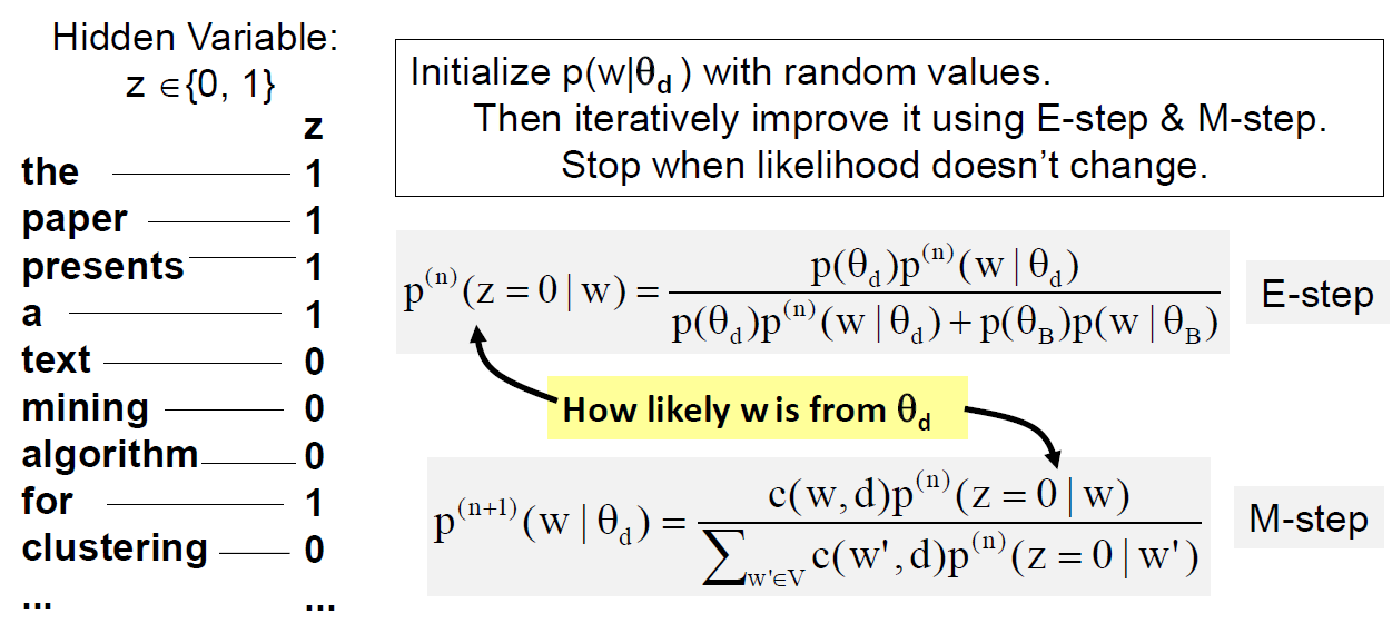
The Expectation-Maximization (EM) Algorithm

• In all the EM algorithms, we introduce a hidden variable to help us solve the problem more easily. Of course we can't observe these z values(that's why we call these hidden variables) and we just imagine the values of z attaching to other words.
• 여기서는 hidden variable이 d과 B로 binary variable로 표현되지만, Topic modeling에서는 hidden variable이 여러개 존재할 수 있다.
• 처음에 each word마다 z value가 0(d)인지 1(B)인지 알 수 없지만, E-Step을 거친 후에 얻은 P(z=0|w)의 확률 값으로 알아볼 수 있다. ( 만약, P(z=0|wi)=0.5이상이면 해당 word i는 z=0으로 할당되었다고 추측해 볼 수 있다. 보통 Iteration 1회 때 z=0인지 z=1인지 분간이 가진다. Background distribution 때문에.. 그 뒤로는 큰 변함이 없다가 converge된다. 예를 들어 background distribution에서 the의 분포가 0.7이면 topic distribution에서 the의 분포가 0.3이하로 낮게 나올 수밖에 없다. (E-Step 방정식 참고))
• [Red Underline] These initialized values would allow us to use the Bayes Rule to take a guess of these z values ( P(z=0|w)의 값에 따라 z value를 알 수 있다. ); 어떤 랜덤 값을 부여하느냐에 따라 모델의 성능이 달라진다. 따라서 EM알고리즘을 multiple time으로 돌려서 global maximum point를 찾는 쪽으로 가야한다.

• [Pink Box] Background distribution은 '소스' 같은 역할.. 매 E-Step마다 Background distribution을 참고해서 P(z=0|w)를 구하고, 즉 다시 Topic distribution을 update한다. Background distribution을 미리 정의해줌으로써 Topic distribution의 특히, common word는 어떻게 형성될건지도 결정된다. ( Topic distribution의 unique word는 주로 count를 통해 split된다. )
• [Orange Box] Since we don't know exactly whether it's 0 or 1, we're not going to really split in a hard way, rather we're going to do a softer split ( we're going to adjust the count by probability that would believe this word has been generated by using the d. ( count를 확률에 반영해 topic 분포의 unique word의 확률을 높여준다 .) )
• [ E-step ] to augment the data with additional information, like z values.
• [ M-step ] to take advantage of the inferred z values and just group words that are in the same distribution and we can normalize the count to estimate the probabilities or to revise our estimate of the parameters.
• We're going to E-step, M-step again, again to improve our estimate of the hidden variables.

EM Computation in Action

• " n " : indicates the generation of parameters.
• " n->n+1 " : means that we have an improvement ( 새로운 observation을 보고 update )

• [Orange Box] 이미 알고 있는 parameters; these are based on a hypothetical corpus; there are several ways to estimate the background language model given a corpus; one common way is to consider all the corpus as 'one document'
• [Blue Box] First, we initialize all the probabilities that are normalized into a uniform distribution.
• [Green Box] E-step would give us a guess of the distribution that has been used to generate each word; 이제 each word마다 서로 다른 확률을 가진다 because these words have different probabilities in the background.
• [Pink Box] now, these words are believed to be more likely from the topic.
• If p(z=0 |wi) is 1.0, then we just use full count of this word i for this topic ( c(w,d)*p(z=0|wi) ); 확률이 1.0이면 모든 count를 반영하겠다.
• 즉, E-step에서 분모에 있는 p(B)*p(topic_word|B) 때문에 p(z=0|topic_word)가 높아진다. 그리고, M-step에서 분자에 있는 c(w,d)*p(z=0|topic_word)의 높은 확률을 가진 p(z=0|topic_word)때문에 p(topic_word|d)가 높아진다. 2단계 모두 topic distribution의 word들의 확률을 최대한 높이려고 해준다.
• In general, it's not going to be 1.0 so, we're going to get some percentage of this count toward this topic and then we simply normalize these counts to have a new generation of parameters estimate.
• Log-Likelihood is negative because the probability is between 0 and 1 when you take a logarithm.
• 마지막 Iteration 3의 p(w|d)와 p(z=0|w)를 해석하는 것은 의미있는 일이다 because our main goal is to estimate these word distribution and we hope to have a more discrimination; 무엇보다 각각 word들의 대한 Topic distribution을 알 수 있다. 

EM as Hill-Climbing ( Converge to Local Maximum )

Hill-Climbing can gradually improve the estimate of parameters and there is some guarantee for reaching a local maximum of the Log-likelihood.

• Start with random guess and by maximizing the lower bound, we'll move this point(current guess) to the top(next guess).
• Since it's a lower bound, we're guaranteed to improve this guess.
• Once we improve our lower bound, and then the original likelihood curve which is above this lower bound, will definitely be improved as well.
• 초기지점을 어떻게 결정하느냐가 중요한데(global 언덕에 갇혀야 하니까), random으로 결정되므로 multiple time으로 돌리는게 낫다; When we have many local maximum, we have to repeat the EM algorithm multiple times in order to pick out which one is the actual global maximum and this is a difficult problem in numerical optimization.